Forces

Here we illustrate how to define and work with forces, using the atomsmltr.environment.fields.forces subpackage.

Note: since MagneticField and Force objects both derive from the Field parent class, all the methods shown in the magnetic field usage tutorial to plot and manipulate magnetic field will also work with forces

Include a constant force (gravity)

Initialize the force

from atomsmltr.environment import ConstantForce
from atomsmltr.atoms import Ytterbium

# let's add gravity, pointing along -z
m = Ytterbium().mass  # kg
g = 9.91  # m/s^2
grav_force = (0, 0, - m * g)
gravity = ConstantForce(field_value=grav_force, tag="gravity")

# print infos
gravity.print_info()

──────────────────
| Constant force |
──────────────────
. Parameters :
  ├── type : constant field
  ├── tag : gravity
  ├── field_value (N) : [ 0.00000000e+00  0.00000000e+00 -2.86234658e-24]
  └── norm (N) : 2.86e-24

Check in a simulation

# -- imports
# atomsmltr
from atomsmltr.environment import ConstantForce
from atomsmltr.atoms import Ytterbium
from atomsmltr.simulation import Configuration, RK4

# other
import numpy as np
import matplotlib.pyplot as plt

# -- config
# init
config = Configuration(atom=Ytterbium())
# add force
m = Ytterbium().mass  # kg
g = 9.91  # m/s^2
grav_force = (0, 0, -m * g)
gravity = ConstantForce(field_value=grav_force, tag="gravity")
config += gravity

# -- simulate
t = np.linspace(0, 1, 1000)
u0 = np.zeros((6,))
res = RK4(config).integrate(u0, t)
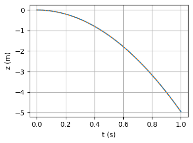
z = res.y[2, :]

# -- plot
plt.figure(figsize=(4, 3), tight_layout=True)
plt.plot(t, z)
plt.plot(t, -0.5 * g * t**2, ":")
plt.grid()
plt.xlabel("t (s)")
plt.ylabel("z (m)")
plt.show()