Polarization maps

The LaserBeam objects allow to get useful information about laser polarization and their projection on a given quantization axis.

Here we illustrate how to use the built-in methods to compute the π, σ+ and σ- components of a laser beam with a given polarization in a complex magnetic field profile.

Simple example : constant offset magnetic field

We start with a constant offset field along x, and a laser with linear polarization along x. In this case we expect the polarization to the π.

import numpy as np
from atomsmltr.environment import GaussianLaserBeam, MagneticOffset
from atomsmltr.environment import CircularLeft, CircularRight, Linear

# - laser beam propagating along +z, linearly polarized along x
laser = GaussianLaserBeam(direction=(0, 0, 1))
laser.polarization = Linear(angle=0)

# - offset beam along x
mag_field = MagneticOffset((1,0,0))

# - then the laser is π-polarized
B = mag_field.get_value((0,0,0))  # value of the field at origin

# compute the norm of the projection on π, σ+- components
# here we use the 'get_polarization_quant_dict' that returns a dict
print("Norm \n------")
components = laser.get_polarization_quant_dict(B)
for k, v in components.items():
    print(f"{k} > {v:.2f}")

# it is also possible to get the projection (complex)
print("\nAmplitude \n------")
components_amp = laser.get_polarization_quant_amplitude_dict(B)
for k, v in components_amp.items():
    print(f"{k} > {v:.2f}")

Norm 
------
sigma+ > 0.00
sigma- > 0.00
pi > 1.00

Amplitude 
------
sigma+ > 0.00+0.00j
sigma- > -0.00+0.00j
pi > 1.00+0.00j

Now if the laser is polarized along y, we have a σ polarization, i.e. a linear superposition of σ- and σ+ :

# update laser polarization
laser.polarization = Linear(np.pi/2)

# norm
print("Norm \n------")
components = laser.get_polarization_quant_dict(B)
for k, v in components.items():
    print(f"{k} > {v:.2f}")

# amplitude
print("\nAmplitude \n------")
components_amp = laser.get_polarization_quant_amplitude_dict(B)
for k, v in components_amp.items():
    print(f"{k} > {v:.2f}")

Norm 
------
sigma+ > 0.50
sigma- > 0.50
pi > 0.00

Amplitude 
------
sigma+ > 0.00-0.71j
sigma- > -0.00+0.71j
pi > 0.00-0.00j

Finally, let’s have the magnetic field aligned with laser propagation, and check that circular polarization correspond to σ+ and σ- polarizations.

# Update magnetic field
mag_field.field_value = (0,0,1)
B = mag_field.get_value((0,0,0))

# Circular right
laser.polarization = CircularRight()
print("Circular right \n------")
components = laser.get_polarization_quant_dict(B)
for k, v in components.items():
    print(f"{k} > {v:.2f}")

# Circular left
laser.polarization = CircularLeft()
print("\nCircular left \n------")
components = laser.get_polarization_quant_dict(B)
for k, v in components.items():
    print(f"{k} > {v:.2f}")

Circular right 
------
sigma+ > 1.00
sigma- > 0.00
pi > 0.00

Circular left 
------
sigma+ > 0.00
sigma- > 1.00
pi > 0.00

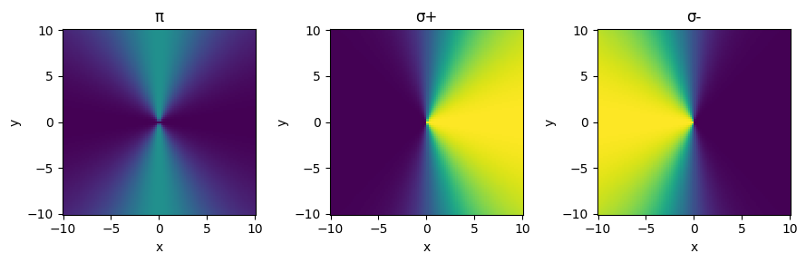
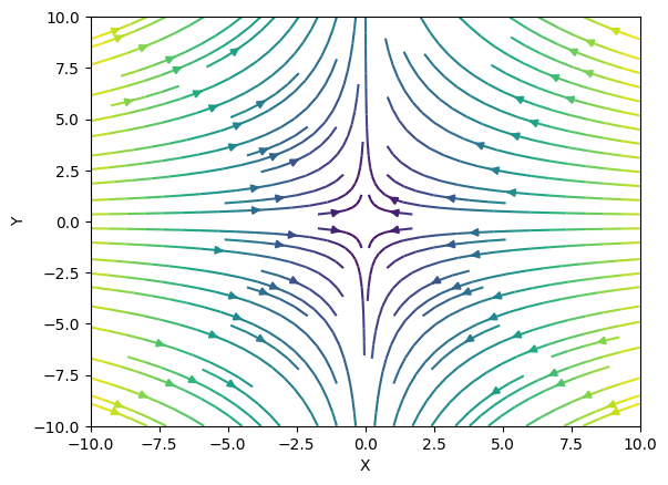
Complex example : polarization map

Now let’s apply this method to compute the polarization projection on a complex magnetic field map.

import numpy as np
import matplotlib.pyplot as plt
from atomsmltr.environment import GaussianLaserBeam, MagneticQuadrupoleX
from atomsmltr.environment import CircularLeft

# - define the magnetic field and laser beam
mag_field = MagneticQuadrupoleX(origin=(0,0,0), slope=1)
laser = GaussianLaserBeam(direction=(1,0,0), polarization=CircularLeft())

# - plot the magnetic field
_ = mag_field.plot2D((-10, 10, -10, 10), (100, 100), plane="XY")

# - compute and plot the polarization map
# prepare grid
position = np.squeeze(np.mgrid[-10:10:100j, -10:10:101j, 0:0:1j]).T

# compute magnetic field value
B = mag_field.get_value(position)

# compute projection
quant = laser.get_polarization_quant(B)
pi, sigma_plus, sigma_minus = quant.T

# plot
X, Y, _ = position.T
fig, axes = plt.subplots(1, 3, figsize=(9, 3), tight_layout=True)

axes[0].pcolormesh(X, Y, pi, vmin=0, vmax=1)
axes[0].set_title("π")
axes[1].pcolormesh(X, Y, sigma_plus, vmin=0, vmax=1)
axes[1].set_title("σ+")
axes[2].pcolormesh(X, Y, sigma_minus, vmin=0, vmax=1)
axes[2].set_title("σ-")

for ax in axes:
    ax.set_ylabel("y")
    ax.set_xlabel("x")
plt.show()