Thermal beam generation#
Here we use atomsmltr for a rather simple example: illustrate the generation of a thermal beam of atoms using a collimation tube.
Context#
We start from an oven containing a gas of atoms of mass \(m\) with a temperature \(T\). According to Boltzmann’s law, the probability distribution for each component \((v_x, v_y, v_z)\) of the speed is given by :
that is a normal distribution with \(\sigma = \sqrt{k_B T / m}\). The oven has a single cylinder-shaped opening, with a radius \(r\) and a length \(L\), that will collimate the beam.
In the following, we will also use Boltzmann’s speed norm distribution \(f_\mathrm{Btz, norm}(v) \equiv P_\mathrm{Btz}(|\vec{v}| = v)\), given by :
Finally, when collimating a beam with a tube of diameter \(d\) and of length \(L\), we expect the following axial velocity distribution (TODO : compute good normalization) :
Simulation#
We will simulate this situation using zones to select atoms that can exit the oven through the tube. This way of solving the problem is arguably overkill, but why not ?
Imports#
# -- atomsmtlr imports
from atomsmltr.simulation import Configuration, RK4
from atomsmltr.atoms import Ytterbium
from atomsmltr.environment import Box, Cylinder, Limits, LowerLimit

# -- other imports
import matplotlib.pyplot as plt
import numpy as np
import scipy.constants as csts
from IPython.display import display, clear_output
from scipy.stats import norm
Generate a thermal distribution#
Let’s start by defining some functions to generate thermal distributions
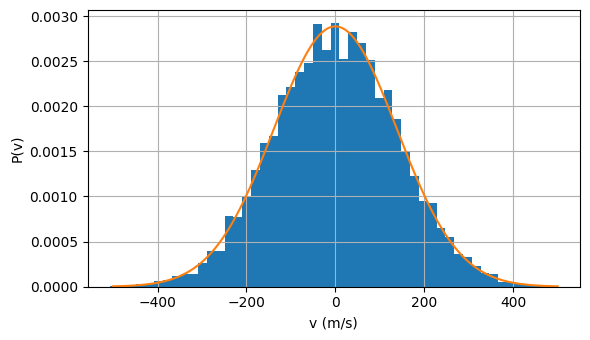
# %% 1D DISTRIBUTION


# - functions
def gen_1D_speed_distrib(N, T, m):
    """Generates a 1D thermal speed distribution,
    with N samples, a temperature T (K) and a mass m (kg)
    """
    rng = np.random.default_rng()
    sigma = np.sqrt(csts.k * T / m)
    v = rng.normal(0, sigma, N)
    return v


def f_Btz(v, T, m):
    """Boltzmann distribution for speed v (m/s)
    temperature T (K) and mass m (kg)
    """
    prefac = np.sqrt(m / 2 / np.pi / csts.k / T)
    exp = np.exp(-m * v**2 / 2 / csts.k / T)
    return prefac * exp

# - test
# settings
T = 400
m = Ytterbium().mass
N = 10_000
# generate
v = gen_1D_speed_distrib(N, T, m)
v_list = np.linspace(-500, 500, 1000)
# plot
plt.figure(figsize=(6, 3.5), tight_layout=True)
plt.hist(v, bins=50, density=True)
plt.plot(v_list, f_Btz(v_list, T, m))
plt.grid()
plt.xlabel("v (m/s)")
plt.ylabel("P(v)")
plt.show()
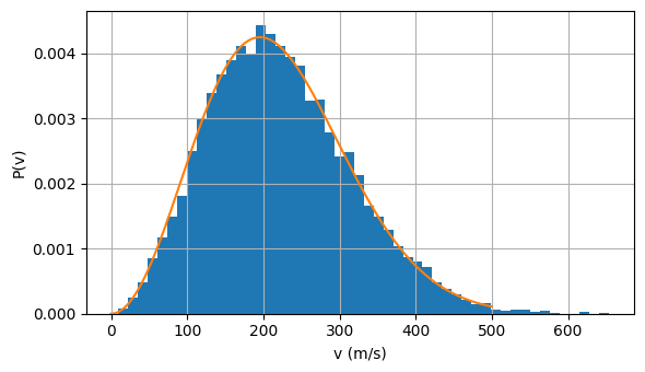
# %% 3D DISTRIBUTION


# - functions
def gen_3D_speed_distrib(N, T, m):
    """Generates a 3D thermal speed distribution,
    with N samples, a temperature T (K) and a mass m (kg).

    Returns an array of shape (N, 3), according to our
    spatial coordinate conventions.
    """
    vx = gen_1D_speed_distrib(N, T, m)
    vy = gen_1D_speed_distrib(N, T, m)
    vz = gen_1D_speed_distrib(N, T, m)
    v = np.array([vx, vy, vz]).T
    return v


def f_Btz_norm(v, T, m):
    """Boltzmann norm distribution in 3D, for speed norm v (m/s)
    temperature T (K) and mass m (kg)
    """
    prefac = 4 * np.pi * (m / 2 / np.pi / csts.k / T) ** (3 / 2)
    exp = np.exp(-m * v**2 / 2 / csts.k / T)
    return prefac * v**2 * exp


# - test
# settings
T = 400
m = Ytterbium().mass
N = 10_000
# generate
v = gen_3D_speed_distrib(N, T, m)
# compute norm
v_norm = np.linalg.norm(v, axis=-1)
v_list = np.linspace(0, 500, 1000)
# plot
plt.figure(figsize=(6, 3.5), tight_layout=True)
plt.hist(v_norm, bins=50, density=True)
plt.plot(v_list, f_Btz_norm(v_list, T, m))
plt.grid()
plt.xlabel("v (m/s)")
plt.ylabel("P(v)")
plt.show()
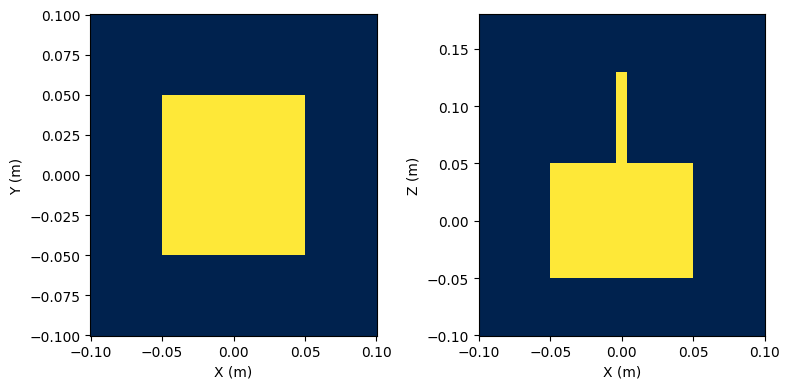
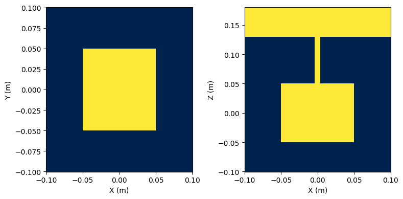
Define configuration with zones#
We will define an experiment zone consisting of :
an oven : a box of dimensions Lx × Ly × Lz
a collimation tube : cylinder of radius r and lenght l, along z
a tube end zone : at the end of the tube, to check if atoms are transmitted.
def gen_zones(Lx, Ly, Lz, r, l):
    """Generates the zones we need for the configuration
    Oven size : Lx * Ly * Lz
    Tube : radius r length l
    """
    # - oven = Box
    oven_dim = (-Lx / 2, Lx / 2, -Ly / 2, Ly / 2, -Lz / 2, Lz / 2)
    oven = Box(*oven_dim, target="position", action="stop", tag="oven")

    # - tube = infinite cylinder & limits
    # cylinder (infinite)
    tube_cyl = Cylinder(
        origin=(0, 0, 0),
        direction=(0, 0, 1),
        radius=r,
        target="position",
        tag="tube cylinder",
    )
    # limits
    tube_lims = Limits(Lz / 2, Lz / 2 + l, axis=2, target="position", tag="tube limits")
    # combine
    tube = tube_cyl & tube_lims
    tube.tag = "tube"
    tube.action = "stop"
    tube.target = "position"

    # - end zone
    end_zone = LowerLimit(
        Lz / 2 + l,
        axis=2,
        target="position",
        action="ignore",
        in_tag="collimated",
        tag="tube end",
    )

    return oven, tube, end_zone


def gen_grid(Lx, Ly, Lz, l):
    # prepare grid
    # xy
    grid_xy = np.mgrid[-Lx:Lx:500j, -Ly:Ly:500j, 0:0:1j]
    grid_xy = np.squeeze(grid_xy)
    X, Y, _ = grid_xy
    X, Y = X.T, Y.T
    pos_xy = grid_xy.T

    # xz
    grid_xz = np.mgrid[-Lx:Lx:500j, 0:0:1j, -Lz : Lz + l : 500j]
    grid_xz = np.squeeze(grid_xz)
    _, _, Z = grid_xz
    pos_xz = grid_xz.T
    Z = Z.T

    return X, Y, Z, pos_xy, pos_xz


# - test
# settings
Lx = Ly = Lz = 10e-2
r = 4e-3
l = 8e-2

# generate
oven, tube, end_zone = gen_zones(Lx, Lz, Ly, r, l)

# print infos
tube.print_info()
oven.print_info()
end_zone.print_info()
───────────────────────
| AND Zone Collection |
───────────────────────
. Parameters :
  ├── type : AND Zone Collection
  ├── tag : tube
  ├── in_tag
  ├── out_tag
  ├── target : position
  ├── action : stop
  ├── zones : ['tube cylinder', 'tube limits']
  └── inverted : False


──────────
| 3D Box |
──────────
. Parameters :
  ├── type : 3D Box
  ├── tag : oven
  ├── in_tag
  ├── out_tag : oven
  ├── target : position
  ├── action : stop
  ├── xmin, xmax : (-0.05, 0.05)
  ├── ymin, ymax : (-0.05, 0.05)
  ├── zmin, zmax : (-0.05, 0.05)
  └── inverted : False


───────────────
| Upper Limit |
───────────────
. Parameters :
  ├── type : 1D lower limit
  ├── tag : tube end
  ├── in_tag : collimated
  ├── out_tag : tube end
  ├── target : position
  ├── action : ignore
  ├── value : 0.13
  ├── axis : 2
  └── inverted : False
# -- plot the zones
# settings
Lx = Ly = Lz = 10e-2
r = 4e-3
l = 8e-2

# generate zones
oven, tube, end_zone = gen_zones(Lx, Lz, Ly, r, l)

# prepare grid
# xy
X, Y, Z, pos_xy, pos_xz = gen_grid(Lx, Ly, Lz, l)

# oven + tube
exp_zone = oven | tube

fig, axes = plt.subplots(1, 2, figsize=(8, 4), tight_layout=True)
axes[0].pcolormesh(X, Y, exp_zone.get_value(pos_xy), cmap="cividis")
axes[0].set_xlabel("X (m)")
axes[0].set_ylabel("Y (m)")
axes[1].pcolormesh(X, Z, exp_zone.get_value(pos_xz), cmap="cividis")
axes[1].set_xlabel("X (m)")
axes[1].set_ylabel("Z (m)")

# oven + tube + end zone
exp_zone = oven | tube | end_zone

fig, axes = plt.subplots(1, 2, figsize=(8, 4), tight_layout=True)
axes[0].pcolormesh(X, Y, exp_zone.get_value(pos_xy), cmap="cividis")
axes[0].set_xlabel("X (m)")
axes[0].set_ylabel("Y (m)")
axes[1].pcolormesh(X, Z, exp_zone.get_value(pos_xz), cmap="cividis")
axes[1].set_xlabel("X (m)")
axes[1].set_ylabel("Z (m)")

plt.show()
Simulation #1 : large tube#
To check our simulation, we start with atoms generated at the center of the oven, and a large tube
# -- Settings
# atoms
m = Ytterbium().mass
T = 400
N = 1000

# geometry
Lx = Ly = Lz = 10e-2
r = 2e-2
l = 8e-2

# duration ?
typical_speed = np.sqrt(csts.k * T / m)
tmax = (l + Lz) / typical_speed * 2
t = np.linspace(0, tmax, 100)

# -- Prepare config
# initial conditions
v = gen_3D_speed_distrib(N, T, m)
vx, vy, vz = v.T
x = np.zeros_like(vx)
y = np.zeros_like(vx)
z = np.zeros_like(vx)

u0 = np.array([x, y, z, vx, vy, vz]).T

# zones
oven, tube, end_zone = gen_zones(Lx, Lz, Ly, r, l)
exp_zone = oven | tube
exp_zone.target = "position"
exp_zone.tag = "exp zone"
exp_zone.action = "stop"
exp_zone.out_tag = "stopped"

# config
config = Configuration(atom=Ytterbium())
config += exp_zone, end_zone

# -- run simulation
sim = RK4(config)
res = sim.integrate(u0, t)
# -- plot resuts : Full trajectory
fig, axes = plt.subplots(1, 2, figsize=(8, 4), tight_layout=True)

# exp zone
X, Y, Z, pos_xy, pos_xz = gen_grid(Lx, Ly, Lz, l)
exp_zone = oven | tube
axes[0].pcolormesh(X, Y, exp_zone.get_value(pos_xy), cmap="Purples_r")
axes[1].pcolormesh(X, Z, exp_zone.get_value(pos_xz), cmap="Purples_r")

# trajectories
y = res.y.T  # shape (len(t), 6, ...)
y = y.reshape((len(res.t), 6, -1))
axes[0].plot(y[:, 0], y[:, 1], "k", linewidth=0.5)
axes[1].plot(y[:, 0], y[:, 2], "k", linewidth=0.5)


# setup
axes[0].set_xlabel("X (m)")
axes[0].set_ylabel("Y (m)")
axes[0].set_xlim(X.min(), X.max())
axes[0].set_ylim(Y.min(), Y.max())
axes[1].set_xlabel("X (m)")
axes[1].set_ylabel("Z (m)")
axes[1].set_xlim(X.min(), X.max())
axes[1].set_ylim(Z.min(), Z.max())
plt.show()
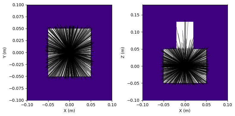
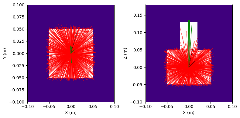
Now let’s use the tags to see what happened to the atoms :
# -- plot resuts : only use last step
fig, axes = plt.subplots(1, 2, figsize=(8, 4), tight_layout=True)

# exp zone
X, Y, Z, pos_xy, pos_xz = gen_grid(Lx, Ly, Lz, l)
exp_zone = oven | tube
axes[0].pcolormesh(X, Y, exp_zone.get_value(pos_xy), cmap="Purples_r")
axes[1].pcolormesh(X, Z, exp_zone.get_value(pos_xz), cmap="Purples_r")

# trajectories
tags = res.tags.T.reshape(-1)
y_last = res.y_last.T.reshape(6, -1)
for tg, u in zip(tags, y_last.T):
    x, y, z, _, _, _ = u
    if "collimated" in tg:
        axes[0].plot((0, x), (0, y), "g", linewidth=1, zorder=3)
        axes[1].plot((0, x), (0, z), "g", linewidth=1, zorder=3)
    elif "stopped" in tg:
        axes[0].plot((0, x), (0, y), "r", linewidth=0.5, zorder=1)
        axes[1].plot((0, x), (0, z), "r", linewidth=0.5, zorder=1)
    else:
        axes[0].plot((0, x), (0, y), "k", linewidth=0.5, zorder=2)
        axes[1].plot((0, x), (0, z), "k", linewidth=0.5, zorder=2)

# setup
axes[0].set_xlabel("X (m)")
axes[0].set_ylabel("Y (m)")
axes[0].set_xlim(X.min(), X.max())
axes[0].set_ylim(Y.min(), Y.max())
axes[1].set_xlabel("X (m)")
axes[1].set_ylabel("Z (m)")
axes[1].set_xlim(X.min(), X.max())
axes[1].set_ylim(Z.min(), Z.max())
plt.show()
Simulation #2 : extract distribution of collimated atoms#
Now we will repeat the experiment and keep only collimated trajectories
# -- Settings for the config
# atoms
m = Ytterbium().mass
T = 400

# geometry
Lx = Ly = Lz = 10e-2
r = 1e-2
l = 8e-2

# zones
oven, tube, end_zone = gen_zones(Lx, Lz, Ly, r, l)
exp_zone = oven | tube
exp_zone.target = "position"
exp_zone.tag = "exp zone"
exp_zone.action = "stop"
exp_zone.out_tag = "stopped"

# config
config = Configuration(atom=Ytterbium())
config += exp_zone, end_zone
We will need a function to perform the simulation on a given speed distribution
Show code cell source
def simulate(tmax, Npoints, Natoms, T, config, start_at_center=True, prefilter=True):
    t = np.linspace(0, tmax, Npoints)

    # -- Prepare config
    # speed
    v = gen_3D_speed_distrib(Natoms, T, m)
    vx, vy, vz = v.T
    # prefilter ?
    if prefilter:
        i = np.logical_and.reduce([vz > 0, np.abs(vz) > np.abs(np.sqrt(vx**2 + vy**2))])
        vx = vx[i]
        vy = vy[i]
        vz = vz[i]
    # position
    if start_at_center:
        x = y = z = np.zeros_like(vx)
    else:
        # get oven zone
        exp_zone = config.get_zone_copy("exp zone")
        for z in exp_zone.zones:
            if z.tag == "oven":
                oven = z
        x = np.random.uniform(oven.xmin, oven.xmax, vx.shape)
        y = np.random.uniform(oven.ymin, oven.ymax, vx.shape)
        z = np.random.uniform(oven.zmin, oven.zmax, vx.shape)
    u0 = np.array([x, y, z, vx, vy, vz]).T

    # -- run simulation
    sim = RK4(config)
    res = sim.integrate(u0, t)

    # -- keep only last
    tags = res.tags.T.reshape(-1).T
    y_last = res.y_last.T.reshape(6, -1).T
    del res
    return y_last, tags
And a function to iterate till we reach a good number of collimated atoms
Show code cell source
def collimate_atoms(N_target, max_iter, *args, **kwargs):
    # -- Simulate
    v_coll = None
    N_gen = 0
    N_coll = 0
    N_flying = 0
    i = 0

    while N_coll < N_target and i < max_iter:
        # simulate
        y, tags = simulate(*args, **kwargs)

        # collected collimated
        coll = np.array(["collimated" in tg for tg in tags])
        not_stopped = np.array(["stopped" not in tg for tg in tags])
        y_coll = y[np.where(coll)]
        if np.sum(coll):
            if v_coll is None:
                v_coll = y_coll[:, 3:]
            else:
                v_coll = np.vstack([v_coll, y_coll[:, 3:]])

        # increment
        N_coll += np.sum(coll)
        N_flying += np.sum(not_stopped)
        N_gen += len(tags)
        i += 1
        x = N_coll / N_target * 100
        clear_output(wait=True)
        display(f"Iteration {i} / {max_iter} | Atoms {N_coll} / {N_target} ({x:.2f}%)")

    del y, tags

    # -- Print
    print("DONE !!")
    print(f"  > collimated atoms   : {N_coll}  ({N_coll / N_gen * 100 :.2f}%) ")
    print(f"  > atoms still flying : {N_flying}  ({N_flying / N_gen * 100 :.2f}%) ")

    res = {"N_coll": N_coll, "N_flying": N_flying, "N_gen": N_gen, "v": v_coll}
    return res
and the theoretical distribution
def f_coll_ax(v, T, m, d, L):
    """axial speed distribution after collimation
    for speed v (m/s), temperature T (K) and mass m (kg)
    with a tube of diameter d (m) and lenght L (m)

    NOTE : normalization is not good
    TODO : compute good normalization
    """
    prefac = np.sqrt(m / 2 / np.pi / csts.k / T)
    exp = np.exp(-m * v**2 / 2 / csts.k / T)
    exp2 = np.exp(-m * v**2 / 2 / csts.k / T * d**2 / L**2)
    return prefac * exp * (1 - exp2)
and a plotting function
Show code cell source
def plot_distrib(res, tube_diameter, tube_length, T, m, show=True):
    # -- preparation
    # get data
    vx, vy, vz = res["v"].T

    # compute theoretical distrib
    v = np.linspace(0, 1000, 1000)
    P = f_coll_ax(v, T, m, tube_diameter, tube_length)
    P /= np.trapezoid(P, v)

    # fit with normal distrib
    mu_x, std_x = norm.fit(vx)
    mu_y, std_y = norm.fit(vy)
    mu_z, std_z = norm.fit(vz)

    # compute
    n = 5
    vx_th = np.linspace(-n * std_x, n * std_x, 1000)
    Px = norm.pdf(vx_th, mu_x, std_x)
    vy_th = np.linspace(-n * std_y, n * std_y, 1000)
    Py = norm.pdf(vy_th, mu_y, std_y)
    vz_th = np.linspace(-n * std_z, n * std_z, 1000)
    Pz = norm.pdf(vz_th, mu_z, std_z)

    # print
    print(f" > vx : mean = {mu_x :.2f} m/s | std = {std_x:.2f} m/s")
    print(f" > vy : mean = {mu_y :.2f} m/s | std = {std_y:.2f} m/s")
    print(f" > vz : mean = {mu_z :.2f} m/s | std = {std_z:.2f} m/s")

    # -- plot
    fig, ax = plt.subplots(1, 3, figsize=(9, 3), tight_layout=True)

    # distributions
    args = {"density": True, "bins": 50}
    ax[0].hist(vx, **args, color="C0")
    ax[0].plot(vx_th, Px, ":k", label="Gaussian")
    ax[0].set_xlabel("v_x (m/s)")
    ax[0].set_xlim(-n * std_x, n * std_x)
    ax[1].hist(vy, **args, color="C1")
    ax[1].plot(vy_th, Py, ":k", label="Gaussian")
    ax[1].set_xlim(-n * std_y, n * std_y)
    ax[1].set_xlabel("v_y (m/s)")
    ax[2].hist(vz, **args, color="C2")
    ax[2].plot(vz_th, Pz, ":k", label="Gaussian")
    ax[2].set_xlabel("v_z (m/s)")

    # theoretical
    ax[2].plot(v, P, "k", label="collimated")
    ax[2].set_xlim(0, 600)

    # gaussians


    for a in ax:
        a.grid()
        a.legend()
    if show:
        plt.show()
    return ax
# -- Settings for simulation
# duration ?
typical_speed = np.sqrt(csts.k * T / m)
tmax = (l + Lz) / typical_speed * 5
N_time = 100

# target
N_target = 5000
N_atoms = 10_000
max_iter = 1000
res = collimate_atoms(
    N_target,
    max_iter,
    tmax,
    N_time,
    N_atoms,
    T,
    config,
    start_at_center=True,
    prefilter=True,
)
'Iteration 302 / 1000 | Atoms 5012 / 5000 (100.24%)'
DONE !!
  > collimated atoms   : 5012  (1.14%)
  > atoms still flying : 49  (0.01%)
# same, atoms spread in oven
N_target = 1000
res_spread = collimate_atoms(
    N_target,
    max_iter,
    tmax,
    N_time,
    N_atoms,
    T,
    config,
    start_at_center=False,
    prefilter=True,
)
'Iteration 502 / 1000 | Atoms 1002 / 1000 (100.20%)'
DONE !!
  > collimated atoms   : 1002  (0.14%)
  > atoms still flying : 58  (0.01%)
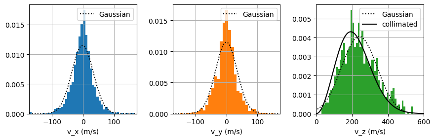
ax = plot_distrib(res, 2 * r, l, T, m)
ax = plot_distrib(res_spread, 2 * r, l, T, m)
 > vx : mean = 0.17 m/s | std = 10.01 m/s
 > vy : mean = -0.28 m/s | std = 10.31 m/s
 > vz : mean = 224.54 m/s | std = 92.97 m/s
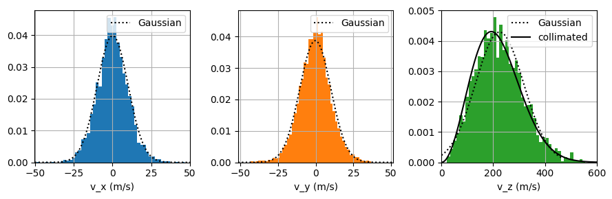
 > vx : mean = -1.48 m/s | std = 34.66 m/s
 > vy : mean = -0.41 m/s | std = 34.73 m/s
 > vz : mean = 240.74 m/s | std = 98.26 m/s