Physical benchmarks: radiation pressure

In this notebook we benchmark atomsmltr simulations on simple physical examples. We focus on the effect of radiation pressure.

Formulaes and orders of magnitude

Radiation pressure

We consider radiation pressure for an atom of mass \(m\), a laser of wavenumber \(k\) and a transition of natural linewidth \(\Gamma\). It takes the form:

\[ F = \hbar k \frac{\Gamma}{2} \frac{s}{1+s}, \]

with \(s\) the saturation parameter, given by:

\[ s = \frac{I}{I_\mathrm{sat}} \frac{1}{1 + (2\delta/\Gamma)^2} \]

where \(I_\mathrm{sat}\) is the transition saturation intensity, and \(\delta\) the laser detuning with respect to the atomic transition. We consider the limit \(s\ll 1\) so that the radiation pressures of independent lasers can be summed up.

Acceleration of an atom at rest

We introduce the typical acceleration due to radiation pressure \(\alpha\), defined as:

\[ \alpha = \frac{\hbar k}{m}\frac{\Gamma}{2} \]

We consider a laser propagating along \(+x\) and an atom initially at rest at \(x=0\). In the limit where \(s\ll 1\), applying Newton’s law of motion we obtain the following trajectory:

\[\begin{split} \left\{ \begin{array}{lr} \ddot{x}(t) = \alpha s\\ \dot{x}(t) = \alpha s t\\ x(t) = \frac{1}{2} \alpha s t^2 \end{array} \right. \end{split}\]

This is valid for short times, that is when the effect of Doppler detuning due to the speed of the atom is negligible. Formally, this means that \(\Delta_\mathrm{Doppler} \equiv k\dot{x} \ll \Gamma\). This yields:

\[ t \ll \frac{2m s}{\hbar k^2} \]

We introduce a typical time \(\tau\):

\[ \tau = \frac{2m}{\hbar k^2} \]

Doppler friction in a 1D Molasse

Now if we consider two counter-propagating beams, in the limit where \(kv \ll \Gamma\), the radiation pressure can be approximated by a friction force :

\[ F_\mathrm{rad} = -m\gamma v \]

with

\[ \gamma = -\frac{\hbar k^2 }{m} s_0 \frac{2 \delta \Gamma}{\delta^2 + \Gamma^2 / 4} \]

where \(s_0 = I / I_\mathrm{sat}\). In this case, an atom with an initial speed \(v_0\) is slowed as \(v(t) = v_0 \exp(-\gamma t)\)

Order of magnitude for the main transition of ytterbium

Let’s give the values of \(\alpha\) and \(\tau\) for the main transition (399nm) of Ytterbium :

# imports
from atomsmltr.atoms import Ytterbium
import scipy.constants as csts

# parameters
atom = Ytterbium()
transition = atom.trans["main"]

# compute
alpha = csts.hbar * transition.k * transition.Gamma / 2 / atom.mass
tau = 2 * atom.mass / csts.hbar / transition.k ** 2
v_friction = transition.Gamma / transition.k

# display
print(f"+ atom mass    : {atom.mass:.3g} kg")
print(f"+ transition Γ : 2π x {transition.Gamma / 2 / csts.pi * 1e-6:.2f} MHz")
print(f"+ transition λ : {transition.wavelength * 1e9:.2f} nm")
print(f"+ transition k : {transition.k * 1e-9:.3f} nm^-1")
print("")
print(f"> acceleration α : {alpha:.2e} m/s^2")
print(f"> recoil speed   : {csts.hbar * transition.k / atom.mass * 1e3:.2f} mm/s")
print(f"> typc. time τ   : {tau * 1e6:.1f} µs")
print(f"> typc. speed v  : {v_friction:.1f} m/s")

+ atom mass    : 2.89e-25 kg
+ transition Γ : 2π x 28.90 MHz
+ transition λ : 398.91 nm
+ transition k : 0.016 nm^-1

> acceleration α : 5.22e+05 m/s^2
> recoil speed   : 5.75 mm/s
> typc. time τ   : 22.1 µs
> typc. speed v  : 11.5 m/s

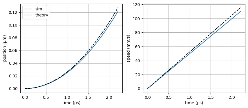
Test #1 : initial acceleration of an atom at rest

We consider the case of an atom initially at rest, at short times - i.e, when the change of detuning due to the Doppler effect is still negligible. We check that the initial acceleration is consistent with the analytical formula.

# - import packages
from atomsmltr.atoms import Ytterbium
from atomsmltr.environment.lasers import PlaneWaveLaserBeam
from atomsmltr.simulation import Configuration, RK4

import matplotlib.pyplot as plt
import numpy as np

# - init config
# atom
atom = Ytterbium()
transition = atom.trans["main"]
transition.print_info()
# laser
s = 0.1
laser = PlaneWaveLaserBeam(
    wavelength=transition.wavelength, direction=(1, 0, 0), tag="399"
)
laser.set_power_from_I(s * transition.Isat)
# config
config = Configuration(atom=atom) + laser
config.add_atomlight_coupling("399", "main", detuning=0)  # resonant laser
# simulator
sim = RK4(config)

# - simulate
# physical parameters
alpha = csts.hbar * transition.k * transition.Gamma / 2 / atom.mass
tau = 2 * atom.mass / csts.hbar / transition.k**2
# simulation parameters
t = np.linspace(0, s * tau, 1_000)
u0 = np.zeros(6)
# run
res = sim.integrate(u0, t)

# - plot results
fig, ax = plt.subplots(1, 2, figsize=(10, 4))
ax[0].plot(res.t * 1e6, res.y[0, :] * 1e6, label="sim")
ax[0].plot(res.t * 1e6, 0.5 * s * alpha * res.t**2 * 1e6, "--k", label="theory")
ax[0].set_ylabel("position (µm)")
ax[0].legend()
ax[1].plot(res.t * 1e6, res.y[3, :] * 1e3)
ax[1].plot(res.t * 1e6, s * alpha * res.t * 1e3, "--k")
ax[1].set_ylabel("speed (mm/s)")

for cax in ax:
    cax.grid()
    cax.set_xlabel("time (µs)")
plt.show()

────────
| main |
────────
. Parameters :
  ├── λ : 398.91 nm
  ├── Γ : 2π × 2.89e+07 Hz
  ├── Isat : 59.51 mw/cm²
  ├── Doppler temp. : 6.93e-04 K
  └── lande factor g : 1.035

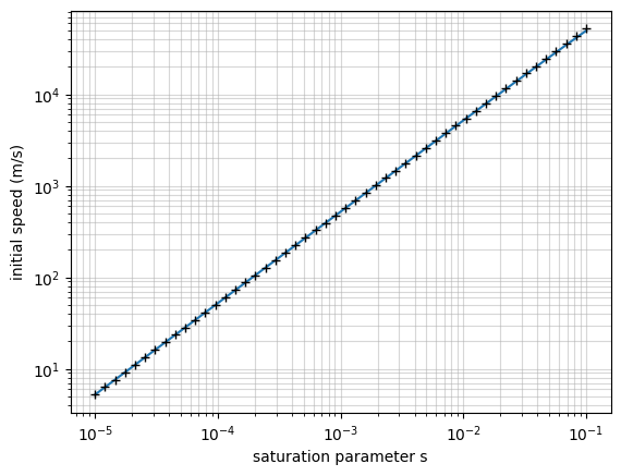
Let’s vary the saturation parameter

s_list = np.logspace(-5, -1, 50)
v0_sim = []

for s in s_list:
    # update laser power
    laser.set_power_from_I(s * transition.Isat)
    config.update_objects(laser)
    sim.config = config
    # run simulation
    t = np.linspace(0, 0.01 * s * tau, 1_000)
    u0 = np.zeros(6)
    res = sim.integrate(u0, t)
    # fit
    p = np.polyfit(res.t, res.y[3,:],deg=1)
    v0_sim.append(p[0])

v0_sim = np.asanyarray(v0_sim)
v0_th = alpha * s_list

plt.figure()
plt.plot(s_list, v0_sim)
plt.plot(s_list, v0_th, '+k')
plt.loglog()
plt.grid(which='both', alpha=0.5)
plt.xlabel("saturation parameter s")
plt.ylabel("initial speed (m/s)")
plt.show()

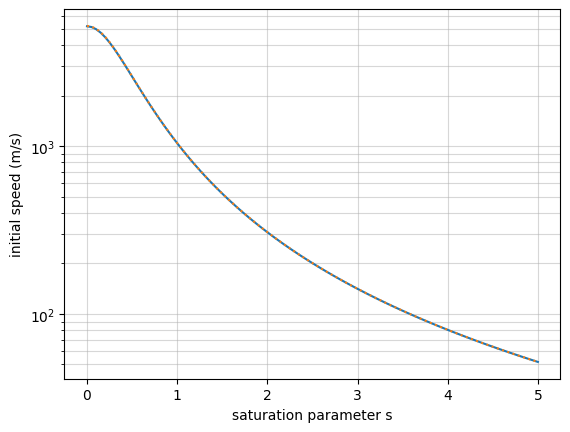
And now let’s change the detuning

s = 0.01
laser.set_power_from_I(s * transition.Isat)
config.update_objects(laser)

delta_list = np.linspace(0, 5, 100)  # in units of Gamma
v0_sim = []

for delta in delta_list:
    # update laser power
    config.reset_atomlight_coupling()
    config.add_atomlight_coupling("399", "main", detuning=delta*transition.Gamma) 
    sim.config = config
    # run simulation
    t = np.linspace(0, 0.01 * s * tau, 1_000)
    u0 = np.zeros(6)
    res = sim.integrate(u0, t)
    # fit
    p = np.polyfit(res.t, res.y[3,:],deg=1)
    v0_sim.append(p[0])

v0_sim = np.asanyarray(v0_sim)
v0_th = alpha * s / (1 + 4 * delta_list ** 2)

plt.figure()
plt.plot(delta_list, v0_sim)
plt.plot(delta_list, v0_th, ':')
plt.semilogy()
plt.grid(which='both', alpha=0.5)
plt.xlabel("saturation parameter s")
plt.ylabel("initial speed (m/s)")
plt.show()

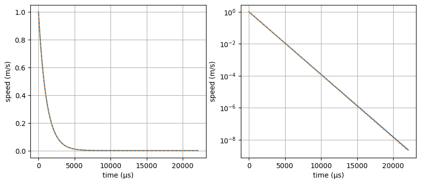
Test #2 : Doppler friction

We now consider an atom with initial speed \(v_0 \ll \Gamma / k\) in a 1D Molasse. For an ytterbium atom on the main transition (399nm), the typical speed is \(\Gamma / k \approx 11\,\mathrm{m/s}\).

# - init config
# atom
atom = Ytterbium()
transition = atom.trans["main"]
transition.print_info()
# lasers
s = 0.01
laser_1 = PlaneWaveLaserBeam(
    wavelength=transition.wavelength, direction=(1, 0, 0), tag="399+"
)
laser_2 = PlaneWaveLaserBeam(
    wavelength=transition.wavelength, direction=(-1, 0, 0), tag="399-"
)
laser_1.set_power_from_I(s * transition.Isat)
laser_2.set_power_from_I(s * transition.Isat)

# config
delta = -0.5 * transition.Gamma
config = Configuration(atom=atom) + laser_1 + laser_2
config.add_atomlight_coupling("399+", "main", detuning=delta)
config.add_atomlight_coupling("399-", "main", detuning=delta)

# simulator
sim = RK4(config)

# - simulate
# physical parameters
k = transition.k
Γ = transition.Gamma
δ = delta
m = atom.mass
gamma = - csts.hbar * k ** 2 / m * s * δ * Γ / (δ ** 2 + Γ ** 2 / 4)
tau = 1 / gamma
# simulation parameters
v0 = 1
t = np.linspace(0, 20 * tau, 1_000)
u0 = np.zeros(6)
u0[3] = v0

# run
res = sim.integrate(u0, t)

# - plot results
fig, ax = plt.subplots(1, 2, figsize=(10, 4))
for cax in ax:
    cax.plot(res.t * 1e6, res.y[3, :], label="sim")
    cax.plot(res.t * 1e6, v0 * np.exp(- gamma * res.t), label="sim", dashes=[2,2])
    cax.grid()
    cax.set_xlabel("time (µs)")
    cax.set_ylabel("speed (m/s)")
ax[1].set_yscale("log")
plt.show()

────────
| main |
────────
. Parameters :
  ├── λ : 398.91 nm
  ├── Γ : 2π × 2.89e+07 Hz
  ├── Isat : 59.51 mw/cm²
  ├── Doppler temp. : 6.93e-04 K
  └── lande factor g : 1.035